SECTION 12.
INTEGRATION METHODS
The present section describes a variety of methods for numerical integration in 1, 2 and 3 dimensions. All input and output variables are REAL*8.
SECTION 12.1 INTEGRATION OF THE NORMAL DENSITY
12.1.1 FUNCTION BIV2 AND BIV2U
BIV2 evaluates the lower tail integral of the bivariate normal density which has been normalized to have zero means and unit variances, i.e., from (-infinity,-infinity) to the point (AX,AY). BIV2U evaluates the upper tail integral, i.e., from (AX,AY) to (infinity,infinity). For description of the method see Owen, D.B., "Tables for Computing Bivariate Normal Probabilities," Annals of Mathematical Statistics, 27 (1956), 1075-1090. BIV2 and BIV2U are called as
      ANSLOW=BIV2(AX,AY,R,IER)
      ANSHIGH=BIV2U(AX,AY,R,IER)
where AX and AY are the upper limits of integration along the X- and Y- axes and R is the correlation between X and Y.
IER = 0 is normal return.
IER =-3 indicates input error (i.e., R is greater than or equal
to 1.0 in absolute value).
12.1.2 FUNCTIONS DUTT2 AND DUTT3
These compute upper tail integrals for the bivariate and trivariate normal densities normalized to have zero means and unit variances. The method is described in Dutt, J.E., "Numerical Aspects of Multivariate Normal Probabilities in Econometric Methods," Annals of Economic and Social Measurement, 17 (1976). 547-561. The calls are
      ANSWER=DUTT2(AX,AY,R12)
      ANSWER=DUTT3(AX,AY,AZ,R12,R13,R23)
respeectively, where AX, AY, AZ are the lower limits of integration and R12, R13, R23 are the correlations X and Y, X and Z and Y and Z respectively. The correlation matrix is not checked for positive definiteness in DUTT3.
12.1.3 FUNCTIONS CLARK2 AND CLARK3
These compute approximations to the upper tail integrals for the bivariate and trivariate normal densities normalized to have zero means and unit variances. The computations are based on Clark, C.E., "The Greatest of a Finite Set of Random Variables," Operation Research, 9 (1961), 145-162. See also Quandt, R.E., The Econometrics of Disequilibrium, Blackwell. The calls are
      ANSWER=CLARK2(AX,AY,R12)
      ANSWER=CLARK3(AX,AY,AZ,R12,R13,R23)
(see 12.1.2). The correlation matrix is not checked for positive in CLARK3.
SECTION 12.2 NEWTON-COTES INTEGRATION OF GENERAL FUNCTIONS
Newton-Cotes integration in 1, 2, and 3 dimensions over rectangular regions is accomplished by
      CALL NEWCT1(AX,BX,NX,FUNC,ANS,IER)
      CALL NEWCT2(AX,BX,AY,BY,NX,NY,FUNC,ANS,IER)
      CALL NEWCT3(AX,BX,AY,BY,AZ,BZ,NX,NY,NZ,FUNC,ANS,IER)
where
AX, BX, AY, BY, AZ, BZ = lower and upper limits of integration
along the X, Y, Z axes
NX, NY, NZ = number of points of integration (2.LE.NX,NY,NZ.LE.9)
along the three axes
FUNC = the name of the FUNCTION subprogram that evaluates the
integrand, defined as FUNCTION FUNC(X), or FUNCTION FUNC(X,Y), or
FUNCTION FUNC(X,Y,Z). FUNC must be declared in an EXTERNAL
statement in the calling routine.
ANS = the answer will be returned here.
IER = 0 if normal return,
IER =-3 if input error (i.e., if the limits of integration do not
define intervals of positive width).
12.2.1 WEDDLE'S RULE (WEDDLE)
Weddle's Rule is a Newton-Cotes type integral formula (see F. B. Hildebrand, Introduction to Numerical Analysis, McGraw-Hill, 1956). WEDDLE is a univariate integration formula and a 7-point Weddle Rule is used over each of n subintervals. This is accomplished by
CALL WEDDLE(AX,BX,N,FUNC,ANS,IER)
where AX and BX are the lower and upper limits of integration respectively, N is the number of subintervals to be used from AX to BX, FUNC is the name of the function that evaluates the integrand, and ANS will contain the answer. IER = 0 normal return = -3 AX is greater than BX
SECTION 12.3 GAUSS-LEGENDRE INTEGRATION
12.3.1 N-POINT INTEGRATION
N-point integration over rectangular regions in 1, 2, 3 dimensions is accomplished by
      CALL GAULG1(AX,BX,NX,FUNC,ANS,IER)
      CALL GAULG2(AX,BX,AY,BY,NX,NY,FUNC,ANS,IER)
      CALL GAULG3(AX,BX,AY,BY,AZ,BZ,NX,NY,NZ,FUNC,ANS,IER)
where the calling parameters have the same meaning as in SECTION 12.2. Note that here NX, NY, NZ must satisfy 2.LE.NX,NY,NZ.LE.11.
12.3.2 ITERATED GAUSS-LEGENDRE INTEGRATION
The calls are
      CALL GAUSA(AX,BX,N,FUNC,ANS,IER)
      CALL BIINT(AX,BX,AY,BY,N,FUNC,ANS,IER)
      CALL TRINT(AX,BX,AY,BY,AZ,BZ,N,FUNC,ANS,IER)
      CALL QUINT(AX,BX,AY,BY,AZ,BZ,AW,BW,N,FUNC,ANS,IER)
perform in 1, 2, 3, 4 dimensions respectively, N times iterated 2-point Gauss-Legendre integration over the rectangular region given by AX,...,BZ. All calling parameters have the same meaning as in SECTION 12.2, except that no separate N may be specified for the X, Y, and Z dimensions. Warning: N must be even!! Note: In the Lahey compiler compatible version QUINT is called QUINTA
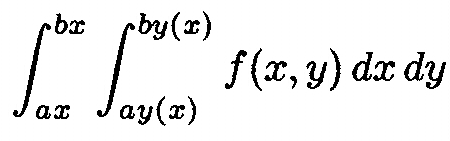
SECTION 12.4 BIVARIATE INTEGRATION WITH VARIABLE LIMITS
1. BIVAR2. The subroutine BIVAR2
performs 10-point Gaussian integration of the function FUNCA(X,Y)
between limits AX and BX along the X-axis and limits AY(X) and
BY(X) along the Y-axis. Hence it computes
The call to BIVAR2 is
CALL BIVAR2(AX,BX,FUNCA,ANS,IER)
where
AX = lower limit along X-axis
BX = upper limit along X-axis
FUNCA = name of function that evaluates the integrand
ANS = contains the answer
IER = 0 if AX .LT. BX and AY(X) .LT. BY(X) and
IER = -3 otherwise. In this latter case no integration is
attempted and the value of ANS is meaningless. The function FUNCA
may be named by the user, but the name must be declared in an
EXTERNAL statement in the MAIN program. It should be defined as
      FUNCTION FUNCA(X,Y)
      IMPLICIT REAL*8 (A-H,O-Z)
       . . . .
      FUNCA=
      RETURN
      END
If the user needs to pass parameters to this function, labelled COMMON should be utilized for the purpose. In addition, the user needs to define two additional functions AY(X) and BY(X) which give the lower and upper limits of integration corresponding to each X-value. These functions should be
      FUNCTION AY(X)
      IMPLICIT REAL*8 (A-H,O-Z)
      AY=
      RETURN
      END
      FUNCTION BY(X)
      IMPLICIT REAL*8 (A-H,O-Z)
      BY=
      RETURN
      END
As before, if these functions require parameters, the user can
pass them via labelled COMMON. As an illustration, consider the
FUNCTION H(X,Y) which is to be integrated from AX to BX along the
X-axis and from 0 to exp(-ax) along
the Y-axis, where H is given by exp(bx)y2: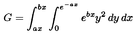
Since the function and the upper Y-limit depend on parameters a and b, they will be passed through labelled COMMON/USER1/A,B. The MAIN program allows the user the input various values of A and B as well as various values of AX and BX. The analytic answer is also computed and is printed along the numerical integral. The listing follows.
      IMPLICIT REAL*8 (A-H,O-Z)
      COMMON/USER1/A,B
      EXTERNAL H
      OPEN (UNIT=9,FILE='BIVAR.DAT',STATUS='OLD')
      READ (9,1000) A,B,AX,BX
1000  FORMAT(4F6.0)
      WRITE (6,1001) A,B,AX,BX
1001  FORMAT(' A,B,AX,BX ',4F8.3)
      TEMP=B-3*A
      C=AX
      D=BX
      TRUTH=1./(3.*TEMP)*(DEXP(TEMP*D)-DEXP(TEMP*C))
      CALL BIVAR2(AX,BX,H,ANS,IER)
      WRITE (*,1002) TRUTH,ANS,IER
1002  FORMAT(' TRUTH,ANS,IER ',2F12.6/1X,I3)
      CLOSE(9)
      STOP
      END
      FUNCTION AY(X)
      IMPLICIT REAL*8 (A-H,O-Z)
      AY=0.
      RETURN
      END
      FUNCTION BY(X)
      IMPLICIT REAL*8 (A-H,O-Z)
      COMMON/USER1/A,B
      BY=DEXP(-A*X)
      RETURN
      END
      FUNCTION H(X,Y)
      IMPLICIT REAL*8 (A-H,O-Z)
      COMMON/USER1/A,B
      H=DEXP(B*X)*Y**2
      RETURN
      END
where the file BIVAR.DAT might contain the line 1.0 1.0 0.0 3.0
2. BIVAR3. BIVAR3 is similar to BIVAR2 with two significant exceptions: (a) Instead of 10-point Gaussian integration, it uses iterated Gauss-Legendre Integration (Section 12.3), where the user can set the number of points of integration arbitrarily; (b) Either or both of the limits AX and BX can be infinite (AX -infinity and/or BX +infinity). The call to BIVAR3 is
CALL BIVAR3(AX,BX,NPT,ICASE,INORM,DELX,DELY,FUNCT,NTR,ANS,IER)
Before we describe the meaning of the various parameters, we need to say a word about how BIVAR3 works when either AX or BX is non-finite. If AX is -infinity, BIVAR3 first computes the bivariate integral over the stripe from BX-DELX to BX; then from BX-2*DELX to B-DELX, etc., until the marginal stripe's integral divided by the sum of the integrals over the previous stripes is less than EPPSS (set at 1.D-8). If AX is finite and BX is + infinity, integration begins over the stripe AX to AX+DELX, then from AX+DEL to AX+2*DELX, and proceeds analogously. If AX is - infinity and BX is +infinity, integration is over pairs of stripes; from 0 to DELX and from -DELX to 0; then from DELX to 2*DELX and from -2*DELX to -DELX, and proceeds analogously to the previous cases. For this to work in any of the three cases, it is important that the integrand be "single peaked;" say we integrate from 0 to +infinity, and DELX = 1; Assume that the integrand is positive from 0 to 1, 0 from 1 to 2, and again positive from 2 to 3. Then BIVAR3 will quit when the upper limit is 2, which is an error. The arguments in the call to BIVAR3 have the following meaning:
AX = lower limit (unless -infinity, in which case it need not
bet set by the user)
BX = upper limit (unless + infinity, in which case it need not be
set by the user)
NPT = Number of point of integration; MUST BE AN EVEN NUMBER
ICASE = 0 both AX and BX are finite and must be specified;
ICASE = 1 AX is -infinity and need not be specified
ICASE = 2 BX is + infinity and need not be specified
ICASE = 3 AX = -infinity, BX = + infinity, and neither needs to
be specified
INORM = 0 if the user will provide a function FUNCT (which must
be declared in an EXTERNAL statement;
INORM = 1 if the integrand is to ve the standard bivariate normal
density function
DELX = width of horizontal stripe (needs to be specified only if
AX or BX is non-finite)
DELY = irrelevant and need not be specified (but a place holder
must be provided for it in the CALL BIVAR3 statement); this is
present for future modifications or if the user wants to provide
for infinite limits in AY(X) or BY(X)
FUNCT = the name of the FUNCTION subprogram that provides the
value of the integrand (must be be defined as FUNCTION FUNCT(X,Y)
and parameters must be passed to it inm labelled COMMON)
NTR = Number of stripe width increases permitted in the initial
stripe until a nonzero integral is obtained (If in the initial
stripe the integral is .LE. 0, the stripe width is increased and
BIVAR3 tries again. A value of 10 might be reasonable.
ANS = the answer
IER = error return;
= 0 for normal return,
= -3 if AX .GE. BX, NPT is not even, or DELX .LE. 0. Note that
appropriate values of DELC and NTR (and also NPT) are problem
dependent, and experimenation with alternative values may be
useful.
SECTION 12.5 UNIVARIATE INTEGRATION OF N(0,1) FROM -INFINITY TO X (DERF)
To compute the integral of the standard normal density from minus infinity to a value x, use
RESULT=0.5+0.5*DERF(X/DSQRT(2.D0)
where both X and RESULT are REAL*8.
SECTION 12.6 ROMBERG INTEGRATION
To compute a univariate integral by Romberg integration, use
CALL ROMB(A,B,EPS,RES,FUNC,IER)
where
A = lower limit
B = upper limit
EPS = tolerance (e.g.,1.D-5)
RES = result
FUNC= name of function evaluating the integrand (must be declared
in an EXTERNAL statement)
IER = error code, = 0 for notmal return
IER =-3 input error (EPS .LE. 0 or A. GE. B)
All real variables must be declared REAL*8. See, for example, Herbert S. Wilf, "Advances in Numerical Quadrature," in Mathematical Methods for Digital Computers, Vol. II, 1966.
SECTION 12.7 GAUSS-LAGUERRE INTEGRATION
To integrate the function f(x) from A to infinity, write a Fortran FUNCTION F(X) which evaluates exp(x)f(x), declare it in an EXTERNAL statement in the calling routine, and
CALL GAUSLA(A,N,F,ANS,IER)
where A, N, F are inputs, ANS, IER are outputs, and
A = lower limit of integration (REAL*8)
N = integer number of points of evaluation (2.LE.N.LE.11)
F = REAL*8 function defined above
ANS = value of the integral (REAL*8)
IER = error code (= 0 normal return, = -3 input error)